1 Introduction

1.1 Probabilistic Models

A probabilistic model consists a sequence of definitions, expressions, and conditions. A model should only use the pure subset of Racket plus the random functions provided by this library.

Here is one of the simplest probabilistic models:

> (flip)

#f

The flip function is a random function that flips a coin (optionally biased) and returns a boolean result.

Random functions can be mixed with ordinary Racket code:

> (repeat (lambda () (flip 0.3)) 10)

'(#f #t #f #f #f #f #f #f #f #t)

Conditions can be expressed using the fail function:

> (unless (for/and ([i 10]) (flip 0.3))     (fail))

fail: failed

Models are typically executed in the context of a sampler or solver designed to explore their probability distribution. The general form is

(sampler/solver-form

def/expr ...

sample-result-expr)

For example, here is a use of rejection-sampler

> (define s-or2flips     (rejection-sampler       (define A (flip))       (define B (flip))       (or A B)))

> (s-or2flips)

#f

> (s-or2flips)

#t

In addition to sampling from random distributions, programs can also perform observations specified by a condition expression using observe/fail. A rejection sampler will simply run the model until it generates a sample satisfying the given condition.

> (define s-first-given-or     (rejection-sampler       (define A (flip))       (define B (flip))       (observe/fail (or A B))       A))

> (s-first-given-or)

#t

> (s-first-given-or)

#t

Samplers can be run multiple times to estimate properties of the probability distributions they represent or to finitely approximate the distribution.

> (sampler->mean+variance s-first-given-or 100 (indicator #t))

71/100 2059/9900

> (sampler->discrete-dist s-first-given-or 100)

(discrete-dist [#f 0.32] [#t 0.68])

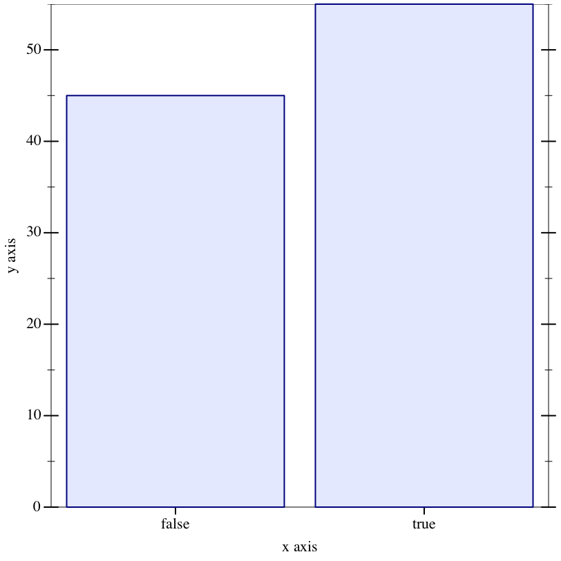
Probability distributions can be visualized with the simple hist function. More comprehensive visualization support is available through the plot library.

> (hist (repeat s-first-given-or 100))

Other sampler and solver forms use more sophisticated techniques to explore the probability distribution represented by a probabilistic model.

1.2 Metropolis-Hastings Sampler

The mh-sampler form implements Metropolis-Hastings sampling.

Here is a simple function that calls flip n times and counts the number of true results:

> (define (count-true-flips n)     (if (zero? n)         0         (+ (if (flip) 1 0)            (count-true-flips (sub1 n)))))

We can define a MH sampler for count-true-flips thus:

> (define s-flips (mh-sampler (count-true-flips 10)))

Calling the sampler produces a sample, but it also records its choices, so that subsequent calls can explore similar sequences of choices. We can use verbose? to see the choices as they’re made.

> (parameterize ((verbose? #t))     (s-flips))

# Starting transition (rerun-mh-transition%) #   NEW (bernoulli-dist 1/2): (1 3 76 79) = 0 #   NEW (bernoulli-dist 1/2): (1 3 76 77 79) = 0 #   NEW (bernoulli-dist 1/2): (1 3 76 77 77 79) = 0 #   NEW (bernoulli-dist 1/2): (1 3 76 77 77 77 79) = 1 #   NEW (bernoulli-dist 1/2): (1 3 76 77 77 77 77 79) = 1 #   NEW (bernoulli-dist 1/2): (1 3 76 77 77 77 77 77 79) = 1 #   NEW (bernoulli-dist 1/2): (1 3 76 77 77 77 77 77 77 79) = 1 #   NEW (bernoulli-dist 1/2): (1 3 76 77 77 77 77 77 77 77 79) = 0 #   NEW (bernoulli-dist 1/2): (1 3 76 77 77 77 77 77 77 77 77 79) = 0 #   NEW (bernoulli-dist 1/2): (1 3 76 77 77 77 77 77 77 77 77 77 79) = 0 # accept threshold = +inf.0 (density dimension +inf.0 -> 0) # Accepted MH step with 0.4725320570372669

4

Each line ends with a series of numbers that identifies the “address” of the call to flip; see [Bher] for details. (Note: if you get a “collision” error, check to make sure your module is using #lang gamble—the language performs call-site instrumentation needed by mh-sampler.)

If we run the sampler again, we see that one of the choices is resampled, and the rest are reused.

> (parameterize ((verbose? #t))     (s-flips))

# Starting transition (single-site-mh-transition%) # key to change = (1 3 76 77 77 77 77 77 79) # DRIFTED from 1 to 0 # PROPOSED from 1 to 0 #   R/F = 1 #   REUSED (bernoulli-dist 1/2): (1 3 76 79) = 0 #   REUSED (bernoulli-dist 1/2): (1 3 76 77 79) = 0 #   REUSED (bernoulli-dist 1/2): (1 3 76 77 77 79) = 0 #   REUSED (bernoulli-dist 1/2): (1 3 76 77 77 77 79) = 1 #   REUSED (bernoulli-dist 1/2): (1 3 76 77 77 77 77 79) = 1 #   PERTURBED (bernoulli-dist 1/2): (1 3 76 77 77 77 77 77 79) = 0 #   REUSED (bernoulli-dist 1/2): (1 3 76 77 77 77 77 77 77 79) = 1 #   REUSED (bernoulli-dist 1/2): (1 3 76 77 77 77 77 77 77 77 79) = 0 #   REUSED (bernoulli-dist 1/2): (1 3 76 77 77 77 77 77 77 77 77 79) = 0 #   REUSED (bernoulli-dist 1/2): (1 3 76 77 77 77 77 77 77 77 77 77 79) = 0 # accept threshold = 1.0 (density dimension 0 -> 0) # Accepted MH step with 0.5381821470665482

3

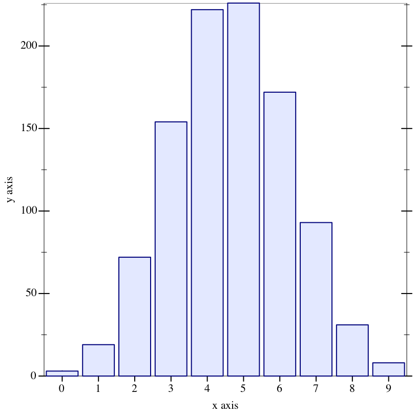
As before, we can use various summarization and visualization functions on the sampler:

> (sampler->mean+variance s-flips 1000)

2469/500 599039/249750

> (sampler->discrete-dist s-flips 1000)

(discrete-dist  [1 0.009]  [2 0.038]  [3 0.125]  [4 0.205]  [5 0.233]  [6 0.215]  [7 0.124]  [8 0.041]  [9 0.009]  [10 0.001])

> (hist (repeat s-flips 1000))

ERP results can be memoized using the mem higher-order function:

> (define s-mem     (mh-sampler       (define mflip (mem (lambda (i) (if (flip) 1 0))))       (for/sum ([i 10]) (mflip (modulo i 5)))))

When we run this sampler, it makes fresh choices for the first five flips, then reuses the memoized choices for the second five flips.

> (parameterize ((verbose? #t))     (s-mem))

# Starting transition (rerun-mh-transition%) #   NEW (bernoulli-dist 1/2): (1 3 89 (mem (0) (88))) = 1 #   NEW (bernoulli-dist 1/2): (1 3 89 (mem (1) (88))) = 1 #   NEW (bernoulli-dist 1/2): (1 3 89 (mem (2) (88))) = 1 #   NEW (bernoulli-dist 1/2): (1 3 89 (mem (3) (88))) = 0 #   NEW (bernoulli-dist 1/2): (1 3 89 (mem (4) (88))) = 0 # accept threshold = +inf.0 (density dimension +inf.0 -> 0) # Accepted MH step with 0.3889577898437205

6

Note: the call to mem must happen in the dynamic extent of the mh-sampler; otherwise, naive memoization will be used instead.

Certain kinds of conditions can be enforced directly using observe-sample, rather than sampling forward and rejecting if the condition is unsatisfied. Indeed, for conditions on continuous random variables, direct enforcement is the only feasible option.

> (define (make-s-cd stddev_R)     (mh-sampler      (define R (normal 10 stddev_R))      (observe-sample (normal-dist R 1) 9)      R))

> (sampler->mean+variance (make-s-cd 3) 1000)

9.108284149869363 0.8823915897092158

> (sampler->mean+variance (make-s-cd 0.5) 1000)

9.781672137575654 0.23369706387681033

1.3 Enumeration via Delimited Continuations

The second technique uses delimited continuations to make a probability-weighted tree of possibile execution paths.

Exhaustive (or nearly exhaustive) exploration of the tree is done with the enumerate solver form.

> (enumerate     (count-true-flips 10))

(discrete-dist  [0 1/1024]  [1 5/512]  [2 45/1024]  [3 15/128]  [4 105/512]  [5 63/256]  [6 105/512]  [7 15/128]  [8 45/1024]  [9 5/512]  [10 1/1024])

The results above agree with the results produced by the binomial distribution:

> (enumerate     (binomial 10 1/2))

(discrete-dist  [0 0.0009765625]  [1 0.009765625000000002]  [2 0.0439453125]  [3 0.11718749999999997]  [4 0.20507812500000006]  [5 0.24609375]  [6 0.20507812500000006]  [7 0.11718749999999997]  [8 0.0439453125]  [9 0.009765625000000002]  [10 0.0009765625])

The enumerate form can be used to approximate countable distributions by using a limit parameter; the tree search stops when the distribution is correct to within the given limit.

> (define (geom)     (if (flip) 0 (add1 (geom))))

> (enumerate     #:limit 1e-06     (geom))

(discrete-dist  [0 524288/1048575]  [1 262144/1048575]  [2 131072/1048575]  [3 65536/1048575]  [4 32768/1048575]  [5 16384/1048575]  [6 8192/1048575]  [7 4096/1048575]  [8 2048/1048575]  [9 1024/1048575]  [10 512/1048575]  [11 256/1048575]  [12 128/1048575]  [13 64/1048575]  [14 32/1048575]  [15 16/1048575]  [16 8/1048575]  [17 4/1048575]  [18 2/1048575]  [19 1/1048575])

Note that the probabilities are not quite the negative powers of 2, because they are normalized after the search stops at 19. Use #:normalize? #f to skip normalization:

> (enumerate     #:limit 1e-06     #:normalize? #f     (geom))

(discrete-measure  [0 1/2]  [1 1/4]  [2 1/8]  [3 1/16]  [4 1/32]  [5 1/64]  [6 1/128]  [7 1/256]  [8 1/512]  [9 1/1024]  [10 1/2048]  [11 1/4096]  [12 1/8192]  [13 1/16384]  [14 1/32768]  [15 1/65536]  [16 1/131072]  [17 1/262144]  [18 1/524288]  [19 1/1048576])

The enumerate form supports memoization through mem:

> (enumerate     (define f (mem (lambda (n) (if (flip) 1 0))))     (list (f 1) (f 2) (f 1) (f 2)))

(discrete-dist  ['(0 0 0 0) 1/4]  ['(0 1 0 1) 1/4]  ['(1 0 1 0) 1/4]  ['(1 1 1 1) 1/4])

The enumerate form supports conditioning:

> (enumerate     #:limit 1e-06     (define A (geom))     (observe/fail (< 20 A 30))     A)

(discrete-dist  [21 256/511]  [22 128/511]  [23 64/511]  [24 32/511]  [25 16/511]  [26 8/511]  [27 4/511]  [28 2/511]  [29 1/511])

Here’s an example from [EPP] that shows that this technique can detect miniscule probabilities that sampling might miss. We disable the limit to explore the tree fully, and we avoid normalizing the resulting probabilities by the acceptance rate of the condition.

> (enumerate    #:normalize? #f    (define (drunk-flip)      (if (flip 0.9)          (fail) ; dropped the coin          (flip 0.05)))    (define (drunk-andflips n)      (cond [(zero? n)             #t]            [else             (and (drunk-flip)                  (drunk-andflips (sub1 n)))]))    (drunk-andflips 10))

(discrete-dist [#f 1.0] [#t 1.0228207236842198e-22])

Enumeration can be nested:

> (enumerate    (define A (flip))    (define B      (enumerate       (define C (flip))       (define D (flip))       (observe/fail (or (and C D) A))       (or C D)))    (list A B))

(discrete-dist  ['(#f #<discrete-dist: [#t 1]>) 1/2]  ['(#t #<discrete-dist: [#f 1/4] [#t 3/4]>) 1/2])

But a memoized function must not be used outside the context that creates it, otherwise an error is raised:

> (enumerate     (define D       (enumerate (mem flip)))     (define f (vector-ref (discrete-dist-values D) 0))     (f))

mem: memoized function escaped its creating context

function: #<procedure:flip>

arguments: '()

The technique of reification and reflection discussed in [EPP] can reduce the complexity of enumerating probabilities. Reification is done using enumerate and reflection with sample. The following pair of programs shows an exponential search tree reduced to a linear one using reification and reflection.

> (define (xor a b) (and (or a b) (not (and a b))))

> (define (xor-flips n)     (if (zero? n)         #t         (xor (flip) (xor-flips (sub1 n)))))

> (time (enumerate (xor-flips 12)))

cpu time: 890 real time: 910 gc time: 771

(discrete-dist [#f 1/2] [#t 1/2])

> (define (xor-flips* n)     (if (zero? n)         #t         (let ([r (sample (enumerate (xor-flips* (sub1 n))))])           (xor (flip) r))))

> (time (enumerate (xor-flips* 12)))

cpu time: 3 real time: 3 gc time: 0

(discrete-dist [#f 1/2] [#t 1/2])

> (time (enumerate (xor-flips* 120)))

cpu time: 38 real time: 39 gc time: 5

(discrete-dist [#f 1/2] [#t 1/2])

Another technique is to delay choices until they are needed. The letlazy function in [EPP] is subsumed by mem. Here’s an example.

> (define (flips-all-true n)     (enumerate       (define Flips (for/list ([i n]) (flip)))       (andmap values Flips)))

> (time (flips-all-true 12))

cpu time: 112 real time: 112 gc time: 25

(discrete-dist [#f 4095/4096] [#t 1/4096])

The search tree has 212 paths, but most of them are redundant because when examining the flip results, we stop looking as soon as we see a #f. By making flips lazy, we only explore a flip when it is actually relevant.

> (define (flips-all-true* n)     (enumerate       (define LFlips (for/list ([i n]) (mem flip)))       (andmap (lambda (f) (f)) LFlips)))

> (time (flips-all-true* 12))

cpu time: 1 real time: 2 gc time: 0

(discrete-dist [#f 4095/4096] [#t 1/4096])

The enumerate solver cannot handle continuous random variables.